When is a Convolutional Filter Easy to Learn

Convolutional Neural Network — II

Continuing our learning from the last post we will be covering the following topics in this post:

• Convolution over volume
• Multiple filters at one time
• One layer of convolution network
• Understanding the dimensional change

I have tried to explain most topics through illustrations as much as possible. If something isn't easy to understand please ping me.

Let's get started!

Convolution over volume

Don't be scared to read 'volume', its just a way of saying images with more than one channel i.e. RGB or any other channels.

Up until now we just had just a single channel so we were just concerned about the height and width of the image. But with the addition of more than one channel we need to take care of the filters involved, as they should also encompass convolution across all channels (3 here).
So if the image dimension is n x n x #channels, so the filter which was earlier f x f would also now be required to be of dimension f x f x #channels.

Intuitively our input data is no more 2 dimensional but in fact 3 dimension if you consider the channels, and hence the name volume.

Below is a simple example of convolution over volume, of an image having dimension 6 x 6 x 3 with 3 denoting the 3 channels R, G and B. Similarly the filter is of dimension 3 x 3 x 3.

Fig 1. Convolution over volume (colour image — 3 channels) with filter of dimension 3 x 3

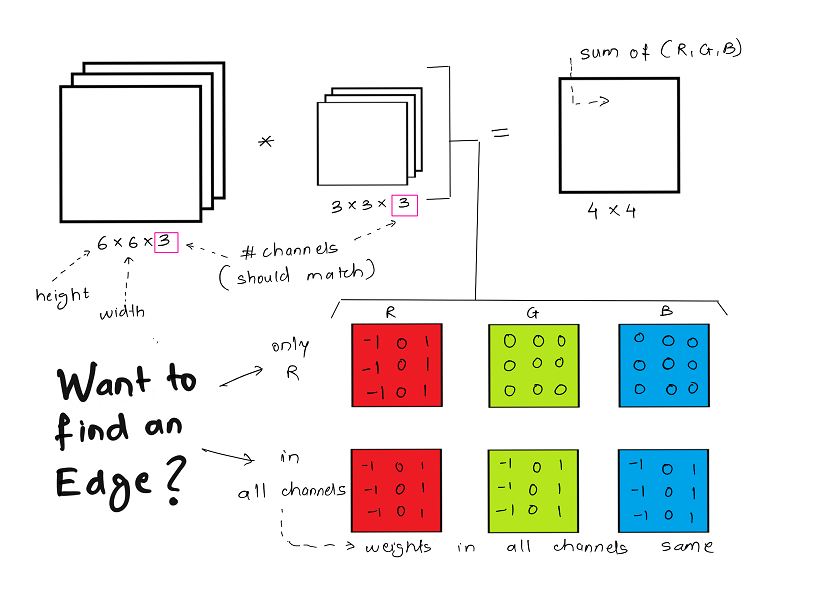
In the given example the purpose of the filter is to detect vertical edges. If the edge needs to be detected only in the R channel,then only the weights in R channel need to set for the requirement. If you need to detect vertical edges across all channels, then all filter channels will have the same weight as demonstrated above.

Multiple filters at one time

There is a high chance that you may need to extract alot of different features from an image, for which you will use multiple filters. If individual filters are convolved separately,it will increase the computation time and so its more convenient to use all required filters at a time directly.

Convolution is carried out individually as is the case with a single filter, and then results of both convolutions are merged together in a stack to form an output volume with a 3rd dimenion representative of the numbers of filters.

Below example considers a 6 x 6 x 3 image as above, but we are using 2 filters ( for vertical edge and horizontal edge) of dimension 3 x 3 x 3. The resultant images of 4 x 4 each are stacked together to get a output volume of 4 x 4 x 2.

Fig 2. Convolution over volume with multiple filter of dimensions 3 x 3

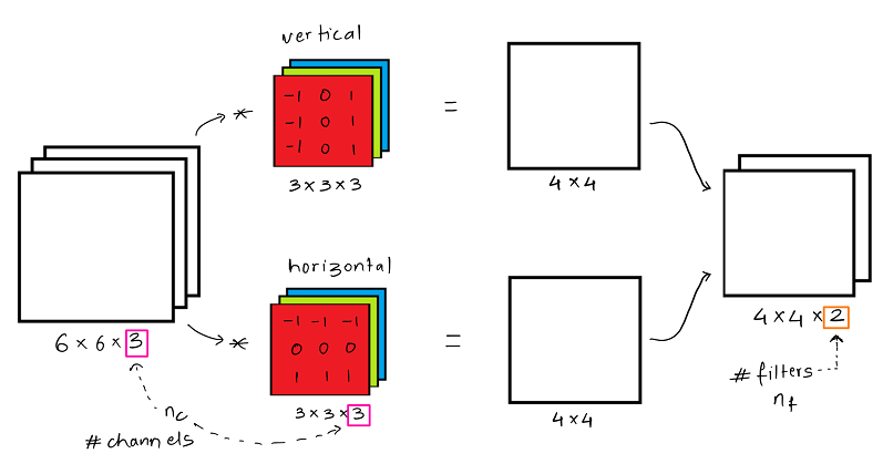
The output dimension can be calculated for any general case using the following equation :

Fig 3. Equation governing the output image/signal dimension wrt input and filter dimension

Here, nc is the number of channels in the input image and nf are the number of filters used.

One layer of convolution network

If we consider one layer of a convolution network without the pooling layer and flattening, then it will appear close to this:

Fig 4. Single layer of convolution network only with Relu activation

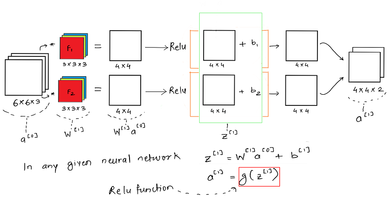
It is important to understand that like in any other neural network, a convolutional neural network also has the input data x which is an image here and model weights given by the filters F1 and F2 i.e. W. Once the weights and the input image is convolved we get the weighted output W * x and then we add the bias b.

One of the key functions here is the RELU activation function, which is rectified linear unit. Relu helps us add non-linearity to the learning model and helps us better train/ learn the model weights for the generalized case.

Fig 5. Relu activation function

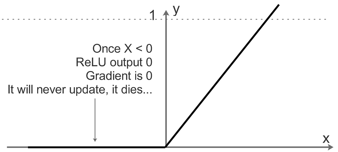
For values which are below a certain threshold ( here 0), the relu function doesn't update the parameters at all. It simply dies. For a particular training example to be considered for training, it needs to have a set minimum value for the neuron to be activated. Also Relu helps us reduce the vanishing and exploding gradient problem faced in most deep neural network, as Relu provides efficient gradient propagation.

Understanding the dimensional change

Now that we have got a conceptual understanding of what is happening in a single layer, lets formulize a outline for a any given layer l of a convolution network.

Fig 6. Equations governing change in input dimensions based on filters, padding and stride

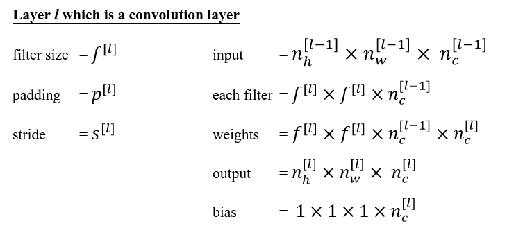
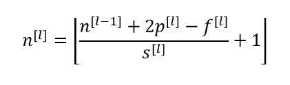
After computing individual components dimension, the final dimension n of layer l can be calculated using:

Fig 7. Dimensions of last layer l with filter size f, padding p and a stride of s

Conclusion

We started this post by exploring convolution over volume and then continued the discussion with multiple filters at once. It easy to understand that the volume here is simply refers to the 3 color channels of the image data. The discussion about a single layer of a convolution network is very vital for grasping the entire network architecture, so make sure these concepts (relu, activation functions) are clear. The final section spoke about how we can assess our model's layer dimension according to the amount of padding and stride used in the convolution with a filter.

In the next post, I will be explaining various CNN architectures in details and assessing its unique features

richardforkildney.blogspot.com

Source: https://towardsdatascience.com/convolutional-neural-network-ii-a11303f807dc

Share this post